博文

Euler-Bernoulli Beam

已有 10639 次阅读 2009-11-26 18:05 |个人分类:英文写作|系统分类:科研笔记

Euler-Bernoulli beam theory (also known as Engineer's beam theory, Classical beam theory or just beam theory) is a simplification of the linear theory of elasticity which provides a means of calculating the load-carrying and deflection characteristics of beams. It was first enunciated circa 1750, but was not applied on a large scale until the development of the Eiffel Tower and the Ferris wheel in the late 19th century. Following these successful demonstrations, it quickly became a cornerstone of engineering and an enabler of the Second Industrial Revolution.

Additional analysis tools have been developed such as plate theory and finite element analysis, but the simplicity of beam theory makes it an important tool in the sciences, especially structural and mechanical engineering.

History

Prevailing consensus is that Galileo Galilei made the first attempts at developing a theory of beams, but recent studies argue that Leonardo da Vinci was the first to make the crucial observations. Da Vinci lacked Hooke's law and calculus to complete the theory, whereas Galileo was held back by an incorrect assumption he made.^[1]

The Bernoulli beam is named after Jacob Bernoulli, who made the significant discoveries. Leonhard Euler and Daniel Bernoulli were the first to put together a useful theory circa 1750.^[2] At the time, science and engineering were generally seen as very distinct fields, and there was considerable doubt that a mathematical product of academia could be trusted for practical safety applications. Bridges and buildings continued to be designed by precedent until the late 19th century, when the Eiffel Tower and Ferris wheel demonstrated the validity of the theory on large scales.

The beam equation

The Euler-Bernoulli equation describes the relationship between the beam's deflection and the applied load:

$frac{partial^2}{partial x^2}left(EI frac{partial^2 u}{partial x^2}right) = w.,$

The curve $u (x)$ describes the deflection $u$ of the beam at some position $x$ (recall that the beam is modeled as a one-dimensional object). $w$ is a distributed load, in other words a force per unit length (analogous to pressure being a force per area); it may be a function of $x$ , $u$ , or other variables.

Note that $E$ is the elastic modulus and that $I$ is the second moment of area. $I$ must be calculated with respect to the centroidal axis perpendicular to the applied loading. For an Euler-Bernoulli beam not under any axial loading this axis is called the neutral axis.

Often, $u = u (x)$ , $w = w (x)$ , and EI is a constant, so that:

$EI frac{d^4 u}{d x^4} = w(x).,$

This equation, describing the deflection of a uniform, static beam, is very common in engineering practice.

Successive derivatives of $u$ have important meanings:

$textstyle{u},$ is the deflection.

$textstyle{frac{partial u}{partial x}},$ is the slope of the beam.

$textstyle{EIfrac{partial^2 u}{partial x^2}},$ is the bending moment in the beam.

$textstyle{-frac{partial}{partial x}left(EIfrac{partial^2 u}{partial x^2}right)},$ is the shear force in the beam.

Stress

Besides deflection, the beam equation describes forces and moments and can thus be used to describe stresses. For this reason, the Euler-Bernoulli beam equation is widely used in engineering, especially civil and mechanical, to determine the strength (as well as deflection) of beams under bending.

Both the bending moment and the shear force cause stresses in the beam. The stress due to shear force is maximum along the neutral axis of the beam (when the width of the beam, t, is constant along the cross section of the beam; otherwise an integral involving the first moment and the beam's width needs to be evaluated for the particular cross section), and the maximum tensile stress is at either the top or bottom surfaces. Thus the maximum principal stress in the beam may be neither at the surface nor at the center but in some general area. However, shear force stresses are negligible in comparison to bending moment stresses in all but the stockiest of beams as well as the fact that stress concentrations commonly occur at surfaces, meaning that the maximum stress in a beam is likely to be at the surface.

It can be shown that the tensile stress experienced by the beam may be expressed as:

$sigma = frac{Mc}{I} = E c frac{partial^2 u}{partial x^2}.,$

Here, $c$ , a position along $u$ , is the distance from the neutral axis to a point of interest; and $M$ is the bending moment. Note that this equation implies that "pure" bending (of positive sign) will cause zero stress at the neutral axis, positive (tensile) stress at the "top" of the beam, and negative (compressive) stress at the bottom of the beam; and also implies that the maximum stress will be at the top surface and the minimum at the bottom. This bending stress may be superimposed with axially applied stresses, which will cause a shift in the neutral (zero stress) axis.

Boundary considerations

The beam equation contains a fourth-order derivative in $x$ , hence it mandates at most four conditions, normally boundary conditions. The boundary conditions usually model supports, but they can also model point loads, moments, or other effects.

A cantilever beam.

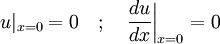
An example is a cantilever beam: a beam that is completely fixed at one end and completely free at the other. "Completely fixed" means that at the left end both deflection and slope are zero; "completely free" implies (though it may or may not be obvious) that at the right end both shear force and bending moment are zero. Taking the $x$ coordinate of the left end as $0$ and the right end as $L$ (the length of the beam), these statements translate to the following set of boundary conditions (assume $E I$ is a constant):

$u|_{x = 0} = 0 quad?; quad frac{partial u}{partial x}bigg|_{x = 0} = 0 qquad mbox{(fixed end)},$
$frac{partial^2 u}{partial x^2}bigg|_{x = L} = 0 quad?; quad frac{partial^3 u}{partial x^3}bigg|_{x = L} = 0 qquad mbox{(free end)},$

Some commonly encountered boundary conditions include:

$textstyle{u = frac{partial u}{partial x} = 0},$ represents a fixed support.

$textstyle{u = frac{partial^2 u}{partial x^2} = 0},$ represents a pin connection (deflection and moment fixed to zero).

$textstyle{frac{partial^2 u}{partial x^2} = frac{partial^3 u}{partial x^3} = 0},$ represents no connection (no restraint) and no load.

$textstyle{-frac{partial}{partial x}left(EIfrac{partial^2 u}{partial x^2}right)} = F,$ represents the application of a point load F.

Loading considerations

Applied loading may be represented either through boundary conditions or through the distributed function $w$ . Using distributed loading is often favorable for simplicity. Boundary conditions are, however, often used to model loads depending on context; this practice being especially common in vibration analysis.

By nature, the distributed load is very often represented in a piecewise manner, since in practice a load isn't typically a "nice" continuous function. Point loads can be modeled with help of the Dirac delta function. For example, consider a static uniform cantilever beam of length $L$ with an upward point load $F$ applied at the free end. Using boundary conditions, this may be modeled through:

$EI frac{d^4 u}{d x^4} = 0,$
$u|_{x = 0} = 0 quad?; quad frac{d u}{d x}bigg|_{x = 0} = 0,$
$frac{d^2 u}{d x^2}bigg|_{x = L} = 0 quad?; quad -EI frac{d^3 u}{d x^3}bigg|_{x = L} = F,$

Using the Dirac function,

$EI frac{d^4 u}{d x^4} = F delta(x - L),$
$u|_{x = 0} = 0 quad?; quad frac{d u}{d x}bigg|_{x = 0} = 0,$
$frac{d^2 u}{d x^2}bigg|_{x = L} = 0,$

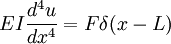
Note that shear force boundary condition (third derivative) is removed, otherwise there would be a contradiction. These are equivalent boundary value problems, and both yield the following solution:

$u = frac{F}{6 EI}(3 L x^2 - x^3),$

The application of several point loads at different locations will lead to $u (x)$ being a piecewise function. Use of the Dirac function greatly simplifies such situations; otherwise the beam would have to be divided into sections, each with four boundary conditions solved separately. A well organized family of functions called Singularity functions are often used as a shorthand for the Dirac function, its derivative, and its antiderivatives.

Clever formulation of the load distribution allows for many interesting phenomena to be modeled. As an example, the vibration of a beam can be accounted for by using the load function:

$w(x, t) = -mu frac{partial^2 u}{partial t^2},$

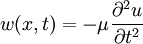
where $μ$ is the linear mass density of the beam, not necessarily a constant. With this time-dependent loading, the beam equation will be a partial differential equation:

$mu frac{partial^2 u}{partial t^2} + frac{partial^2}{partial x^2} left( EI frac{partial^2 u}{partial x^2} right) = 0.$

Another interesting example describes the deflection of a beam rotating with a constant angular frequency of $ω$ :

$w(u) = mu omega^2 u,$

This is a centripetal force distribution. Note that in this case, $w$ is a function of the displacement (the dependent variable), and the beam equation will be an autonomous ordinary differential equation.

Extensions

The kinematic assumptions upon which the Euler-Bernoulli beam theory is founded allow it to be extended to more advanced analysis. Simple superposition allows for three-dimensional transverse loading. Using alternative constitutive equations can allow for viscoelastic or plastic beam deformation. Euler-Bernoulli beam theory can also be extended to the analysis of curved beams, beam buckling, composite beams, and geometrically nonlinear beam deflection.

Euler-Bernoulli beam theory does not account for the effects of transverse shear strain. As a result it underpredicts deflections and overpredicts natural frequencies. For thin beams (beam length to thickness ratios of the order 20 or more) these effects are of minor importance. For thick beams, however, these effects can be significant. More advanced beam theories such as the Timoshenko beam theory (developed by the Russian-born scientist Stephen Timoshenko) have been developed to account for these effects.

Lagrangian formulation

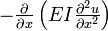
The beam equation is the Euler-Lagrange equation for the following action

$S = int_O^L left( (1/2)mu left( partial u/partial t right)^2 + (1/2)left( EI partial^2 u/partial x^2 right)^2 -w(x) u(x,t)right) dx$

The first term represents the kinetic energy ; the second one is (minus) the potential energy due to internal forces ; the third term is the potential energy due do the external load $w (x)$ .

转载本文请联系原作者获取授权，同时请注明本文来自潘超科学网博客。
链接地址：https://blog.sciencenet.cn/blog-339218-274160.html

上一篇：动力时程分析方法的MATLBA源代码（1）中心差分法
下一篇：Timoshenko beam theory

收藏 IP: .*| 热度|

当前推荐数：0

发表评论评论 (0 个评论)

数据加载中...

返回顶部

博文发布时间已经超过87600小时，评论已关闭。

潘超

扫一扫，分享此博文

超越梦想分享 http://blog.sciencenet.cn/u/pcabaqus 结构减隔震控制非线性抗震分析 Python简单编程

博文

Euler-Bernoulli Beam

Stress

当前推荐数：0

发表评论评论 (0 个评论)

潘超

全部作者的其他最新博文

全部精选博文导读

相关博文

超越梦想分享 http://blog.sciencenet.cn/u/pcabaqus 结构减隔震控制 非线性抗震分析 Python简单编程

博文

Euler-Bernoulli Beam

Stress

当前推荐数：0

发表评论 评论 (0 个评论)

潘超

全部作者的其他最新博文

全部精选博文导读

相关博文

超越梦想分享 http://blog.sciencenet.cn/u/pcabaqus 结构减隔震控制非线性抗震分析 Python简单编程

发表评论评论 (0 个评论)