博文
[转载]Integration by Pullback
||| |
Integration by Pullback
Frank Wang, fwang@lagcc.cuny.edu
The calculus of differential forms is a powerful tool that unifies and simplifies many mathematical concepts. We use the Pullback command in Maple's DifferentialGeometry package to perform double, triple, line and surface integrals in James Stewart's Calculus to demonstrate the method differential forms and show the connection among these integrals.
Like many math professors around the world, I teach from home in the spring semester of 2020 because of the coronavirus pandemic. On March 11, 2020, New York State Governor Andrew Cuomo announced that all public university campuses would be closed. I left my office hastily without a chance to gather my teaching notes. One of the courses I'm teaching is Calculus 3, which covers double and triple integrals, line integrals, and surface integrals. The calculations involved in these types of integrals tend to be lengthy, even for textbook problems. I took the opportunity to rewrite my notes using differential forms with the assistance of Maple. I hope this note will help math instructors double check their their calculations, and perhaps introduce modern concept of differential geometry to students.
A volume integral leads to a 3-form, a line integral leads to a 1-form, and a surface integral leads to a two form; see Flanders' nice book. We will give examples below based on exercises from the popular calculus textbook by James Stewart (8th edition).
Consider two manifolds M and N, possibly of different dimension. A manifold in the present work is simply an n-dimensional Euclidean space. Suppose we have a smooth map f: M -> N. This map induces a map f* from the cotangent space of N to that of M. Because f* goes the opposite direction of f, it's called a pullback.
Imagine that M is a three-dimensional Euclidean space with Cartesian coordinates, and N the same space but with spherical coordinates. We evaluate three triple integrals in Stewart Section 15.8, Exercises 41--43.
restart:
with(DifferentialGeometry): with(plots):
We first define manifolds M and N, and the transformation.
DGsetup([x,y,z], M); DGsetup([rho, theta, phi], N);
frame name: M
frame name: N
f := Transformation(N, M, [x=rho*sin(phi)*cos(theta), y=rho*sin(phi)*sin(theta), z=rho*cos(phi)]);

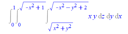
Exercise 41:
Int(Int(Int(x*y, z=sqrt(x^2+y^2)..sqrt(2-x^2-y^2)), y=0..sqrt(1-x^2)), x=0..1);
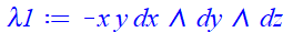
We define a three-form associated with M, and pullback to N.
lambda1 := evalDG(x*y*dz &wedge dy &wedge dx);
l1p := Pullback(f, lambda1);

The triple integral is over the region shown below.
p11 := plot3d([sqrt(2)*sin(phi)*cos(theta), sqrt(2)*sin(phi)*sin(theta), sqrt(2)*cos(phi)], phi=0..Pi/4, theta=0..Pi/2):
p12 := plot3d([rho*sin(Pi/4)*cos(theta), rho*sin(Pi/4)*sin(theta), rho*cos(Pi/4)], rho=0..sqrt(2), theta=0..Pi/2):
display({p11, p12}, scaling = constrained);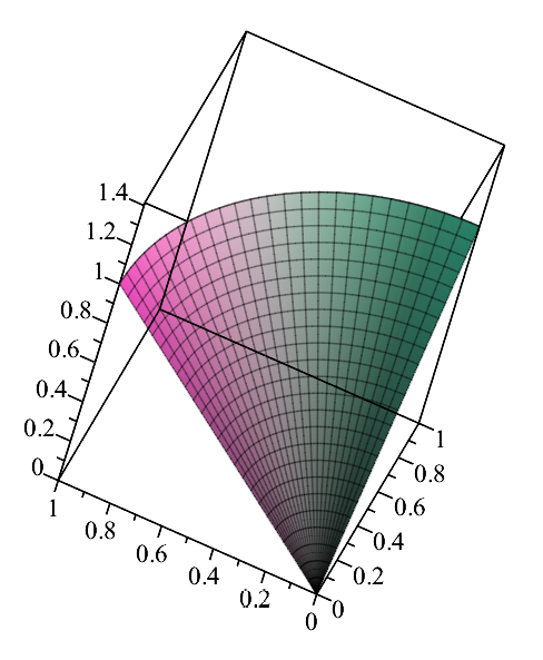
We integrate the three form.
IntegrateForm(l1p, rho=0..sqrt(2), phi=0..Pi/4, theta=0..Pi/2);

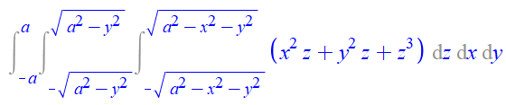
Exercise 42 is below, with a similar procedure as above.
Int(Int(Int(x^2*z+y^2*z+z^3, z=-sqrt(a^2-x^2-y^2)..sqrt(a^2-x^2-y^2)), x=-sqrt(a^2-y^2)..sqrt(a^2-y^2)), y=-a..a);
lambda2 := evalDG((x^2*z+y^2*z+z^3)*dz &wedge dx &wedge dy);

l2p := Pullback(f, lambda2);
The triple integral is over the region of a sphere centered at the origin with radius a.
plot3d([sin(phi)*cos(theta), sin(phi)*sin(theta), cos(phi)], phi=0..Pi, theta=0..2*Pi);

This integral vanishes.
IntegrateForm(l2p, rho=0..a, phi=0..Pi, theta=0..2*Pi);
0
Exercise 43.
Int(Int(Int((x^2+y^2+z^2)^(3/2), z=2-sqrt(4-x^2-y^2)..2+sqrt(4-x^2-y^2)), y=-sqrt(4-x^2)..sqrt(4-x^2)), x=-2..2);

lambda3 := evalDG((x^2+y^2+z^2)^(3/2)*dz &wedge dy &wedge dx);
l3p := Pullback(f, lambda3);

l3p := evalDG(l3p) assuming rho>0;
The triple integral is over the region of a sphere whose center is (0,0,2) and radius 2.
plot3d([2*sin(phi)*cos(theta), 2*sin(phi)*sin(theta), 2*cos(phi)+2], phi=0..Pi, theta=0..2*Pi);

The integration of the three-form is below.
IntegrateForm(l3p, theta=0..2*Pi, phi=0..Pi/2, rho=0..4*cos(phi));
restart:
Before continuing additional examples, let us review an elementary problem in single-variable calculus. Consider Stewart Section 5.5 Substitution Rule Example 1:
Int(x^3*cos(x^4+2), x);
In the textbook students learn the method of setting u=g(x)=x^4+2 and evaluating du=g'(x)dx. Here we consider two one-dimensional manifolds, M and N, with coordinate x and u, respectively.
with(DifferentialGeometry):
DGsetup([x], M); DGsetup([u], N);
frame name: M
frame name: N
The transformation from M to N is the following.
g := Transformation(M, N, [u=x^4+2]);
omega := evalDG(x^3*cos(x^4+2)*dx);

But to pullback from the cotangent space of M to that of N, we need the inverse transformation (hence the name pullback).
ginv := InverseTransformation(g);
![]()
omega1 := Pullback(ginv, omega);
![]()
i1 := IntegrateForm(omega1, u);
![]()
Now we pullback the function (a zero-form) to M.
Pullback(g, i1);
![]()
restart:
The component expression of f* is given by the Jacobian matrix, as illustrated in next problem (Stewart Section 15.9 Exercise 18): evaluate the double integral of the function f(x,y)=x^2-x*y+y^2 over the interior of an ellipse.
plot3d(x^2-x*y+y^2, x=-2..2, y=-2..2);

plots[implicitplot](x^2-x*y+y^2=2, x=-2..2, y=-2..2);

We can use VectorCalculus[int] to find the answer.
with(VectorCalculus):
int(x^2-x*y+y^2, [x,y]=Ellipse(x^2-x*y+y^2-2));
![]()
We go through this calculation in steps. Firstly, we define manifolds M with coordinates (x,y) and N wit coordinates (u,v), and the transformation (given in the textbook).
with(DifferentialGeometry):
DGsetup([x, y], M); DGsetup([u, v], N);
frame name: M
frame name: N
f := Transformation(N, M, [x=sqrt(2)*u-sqrt(2/3)*v, y=sqrt(2)*u+sqrt(2/3)*v]);
![]()
The Jacobian matrix is below.
Tools:-DGinfo(f, "JacobianMatrix");

The two-form in connection with this double integral is below. Using pullback, the two-form is in the space cotangent to N.
alpha := evalDG((x^2 - x*y+y^2)*dx &wedge dy);
![]()
When we pullback the ellipse, we find a unit circle in N.
e := Pullback(f, x^2-x*y+y^2-2);
![]()
expand(e);
![]()
It is apparently more convenient to use polar coordinates. Below is the transformation.
DGsetup([r, theta], M2);
frame name: M2
f2 := Transformation(M2, N, [u=r*cos(theta), v=r*sin(theta)]);
![]()
alpha2 := Pullback(f2, alpha1);
![]()
The integration of the two-form is shown below.
IntegrateForm(alpha2, r=0..1, theta=0..2*Pi);
![]()
restart:
Consider Stewart Section 16.2 Exercise 21, a line integral over a vector field visualized below.
with(plots):
pf := fieldplot3d([sin(x), cos(y), x*z], x=-1..1, y=-1..1, z=-1..1, color = blue):
pc := spacecurve([t^3, -t^2, t], t=0..1, color = red, thickness = 2):
display([pf, pc]);

M is our usual three-dimensional Euclidean space, and N is a one-dimensional manifold with coordinate t.
with(DifferentialGeometry):
DGsetup([x, y, z], M): DGsetup([t], N);
frame name: N
The transformation is the spacecurve given.
f := Transformation(N, M, [x=t^3, y=-t^2, z=t]);
![]()
We define the one-form, and find its pullback.
omega := evalDG(sin(x)*dx + cos(y)*dy + x*z*dz);
![]()
The one-form can be integrated.
IntegrateForm(omega1, t=0..1);
![]()
restart:
The image below is based on the surface integral over a vector field, Stewart Section 16.7 Exercise 28.
with(plots):
pf := fieldplot3d([y*z, z*x, x*y], x=0..2, y=0..Pi, z=0..2, color = red):
ps := plot3d(x*sin(y), x=0..2, y=0..Pi, style = hidden):
display([pf, ps]);

We consider M as the three-dimensional Euclidean space, and N the xy-plane. The graph of z=x*sin(y) is the surface given in the exercise.
with(DifferentialGeometry):
DGsetup([x, y, z], M); DGsetup([x, y], N);
frame name: M
frame name: N
f := Transformation(N, M, [x=x, y=y, z=x*sin(y)]);
![]()
ChangeFrame(M);
N
The following is the two-form and its pullback.
alpha := evalDG(y*z*dy &wedge dz + z*x*dz &wedge dx + x*y*dx &wedge dy);
![]()
alpha1 := Pullback(f, alpha);
![]()
The integration of the two form is below.
IntegrateForm(alpha1, x=0..2, y=0..Pi);
![]()
restart:
Let us work out another surface integral over a vector field, Stewart Section 16.7 Exercise 26.
with(plots):
pf := fieldplot3d([y, -x, 2*z], x=-2..2, y=-2..2, z=0..2, color = red, scaling = constrained):
ps := plot3d([2*sin(phi)*cos(theta), 2*sin(phi)*sin(theta), 2*cos(phi)], phi=0..Pi/2, theta=0..2*Pi, style = hidden, scaling = constrained):
display([pf, ps]);

The transformation below should be familiar.
with(DifferentialGeometry):
DGsetup([x, y, z], M): DGsetup([phi, theta], N):
f := Transformation(N, M, [x=2*sin(phi)*cos(theta), y=2*sin(phi)*sin(theta), z=2*cos(phi)]);
![]()
We define the two-form and find its pullback, then integrate the pullback.
alpha := evalDG(y*dy &wedge dz - x*dz &wedge dx +2*z*dx &wedge dy);
![]()
alpha1 := Pullback(f, alpha);
![]()
IntegrateForm(alpha1, theta=0..2*Pi, phi=0..Pi/2);
![]()
restart:
Stokes' and Divergence Theorems can be elegantly written using differential forms.

We verify Stokes' Theorem as instructed in Stewart Section 16.8. Consider the line integral over a vector field, Exercise 15, where the curve is the boundary of the surface shown below.
with(plots):
pf := fieldplot3d([y, z, x], x=-1..1, y=-1..1, z=-1..1, color=blue):
ps := plot3d([sin(phi)*cos(theta), sin(phi)*sin(theta), cos(phi)], phi=0..Pi, theta=-Pi/2..Pi/2, style = hidden, scaling = constrained):
display({pf, ps});
with(DifferentialGeometry):
Let M be the three-dimensional Euclidean space, N be one dimensional space with coordinate t, and N1 be two-dimensional space with coordinates theta and phi.
DGsetup([x,y,z], M): DGsetup([t], N): DGsetup([theta,phi], N1):
f1 := Transformation(N, M, [x=cos(t), y=0, z=sin(t)]);
![]()
We define the one-form and perform the line integral using pullback as before.
omega := evalDG(y*dx + z*dy + x*dz);
![]()
omega1 := Pullback(f1, omega);
![]()
IntegrateForm(omega1, t=0..2*Pi);
![]()
The curl of a vector corresponds to the exterior derivative of the one form.
alpha := ExteriorDerivative(omega);
![]()
After parametrizing the hemisphere, we pullback the two-form.
f2 := Transformation(N1, M, [x=sin(phi)*cos(theta), y=sin(phi)*sin(theta), z=cos(phi)]);
![]()
alpha1 := Pullback(f2, alpha);
![]()
The integration of the two form over the surface is the same as the line integral above.
IntegrateForm(alpha1, phi=0..Pi, theta=-Pi/2..Pi/2);
![]()
restart:
The figure below is based on Stewart Section 16.8 Exercise 14, another exercise to verify Stokes' Theorem.
with(plots):
pf := fieldplot3d([-2*y*z, y, 3*x], x=-3..3, y=-3..3, z=0..6, color=blue):
ps := plot3d([r*cos(theta), r*sin(theta), 5-r^2], r=0..2, theta=0..2*Pi, style = hidden, scaling = constrained):
display({pf, ps});
with(DifferentialGeometry):
DGsetup([x,y,z], M): DGsetup([t], N): DGsetup([x, y], M1):
f1 := Transformation(N, M, [x=2*cos(t), y=2*sin(t), z=1]);
![]()
We define the one-form and evaluate the line integral using pullback.
omega := evalDG(-2*y*z*dx + y*dy + 3*x*dz);
![]()
omega1 := Pullback(f1, omega);
![]()
IntegrateForm(omega1, t=0..2*Pi);
![]()
The exterior derivative of the one-form corresponds to the curl.
alpha := ExteriorDerivative(omega);
![]()
f2 := Transformation(M1, M, [x=x, y=y, z=5-x^2-y^2]);
![]()
alpha1 := Pullback(f2, alpha);
![]()
It is easier to integrate this two-form using polar coordinates, as shown in the following.
DGsetup([r, theta], N2);
frame name: N2
f3 := Transformation(N2, M1, [x=r*cos(theta), y=r*sin(theta)]);
![]()
alpha2 := Pullback(f3, alpha1);
![]()
We verify Stokes' Theorem.
IntegrateForm(alpha2, r=0..2, theta=0..2*Pi);
![]()
restart:
Below is the surface integral over a given vector field, taken from Stewart Section 16.9 Exercise 4. We will evaluate the surface integral using the Divergence Theorem first, then calculate the surface integrals directly.
with(plots):
pf := fieldplot3d([x^2, -y, z], x=-1..3, y=-3..3, z=-3..3, color = blue, scaling = constrained);

ps1 := plot3d([x, 3*cos(theta), 3*sin(theta)], x=0..2, theta=0..2*Pi, style = hidden);

ps2 := plot3d([0, r*cos(theta), r*sin(theta)], r=0..3, theta=0..2*Pi, style = hidden);

ps3 := plot3d([2, r*cos(theta), r*sin(theta)], r=0..3, theta=0..2*Pi, style = hidden);

display({pf, ps1, ps2, ps3});
with(DifferentialGeometry):
DGsetup([x,y,z], M);
frame name: M
We define the two-form, and the exterior derivative of it corresponds to the divergence of the vector field.
alpha := evalDG(x^2*dy &wedge dz - y*dz &wedge dx + z*dx &wedge dy);
![]()
lambda := ExteriorDerivative(alpha);
![]()
It is more convenient to integrate this three-form using cylindrical coordinates, as demonstrated below.
DGsetup([x, r, theta], N);
frame name: N
f := Transformation(N, M, [x=x, y=r*cos(theta), z=r*sin(theta)]);
![]()
lambda1 := Pullback(f, lambda);
![]()
IntegrateForm(lambda1, x=0..2, r=0..3, theta=0..2*Pi);
![]()
To calculate the surface integral, we need to deal with 3 surfaces. Surfaces 1, 2, and 3 are depicted above in ps1, ps2, and ps3, respectively. The pullback of the two-form for the three surfaces are below.
DGsetup([r, theta], N1); DGsetup([x, theta], N2);
frame name: N1
frame name: N2
f1 := Transformation(N2, M, [x=x, y=3*cos(theta), z=3*sin(theta)]);
![]()
f2 := Transformation(N1, M, [x=0, y=r*cos(theta), z=r*sin(theta)]);
![]()
f3 := Transformation(N1, M, [x=2, y=r*cos(theta), z=r*sin(theta)]);
![]()
alpha1 :=Pullback(f1, alpha);
![]()
alpha2 := Pullback(f2, alpha);
![]()
alpha3 := Pullback(f3, alpha);
![]()
IntegrateForm(alpha1, x=0..2, theta=0..2*Pi);
0
IntegrateForm(alpha2, r=0..3, theta=0..2*Pi);
0
IntegrateForm(alpha3, r=0..3, theta=0..2*Pi);
![]()
The flux across surfaces 1 and 2 is zero, and flux across surface 3 is the same as the integral obtained from the Divergence Theorem.
References
1. James Stewart (2016). Calculus (Early Transcendentals), 8th edition. Boston: Cengage.
2. Harley Flanders (1963). Differential Forms with Applications to the Physical Sciences. New York: Dover.
3. David M. Bressoud (1991). Second Year Calculus. New York: Springer.
https://blog.sciencenet.cn/blog-516836-1244017.html
上一篇:[转载]Maple量子化学工具箱 - 2020版新增功能
下一篇:子弹轨迹模型