博文

对于共轭梯度最优化方法的一些认识

已有 22366 次阅读 2012-5-10 17:24 |个人分类:统计学与R语言学习|系统分类:科研笔记

共轭梯度法最初由Hesteness和Stiefel于1952年为求解线性方程组而提出的。后来，人们把这种方法用于求解无约束最优化问题，使之成为一种重要的最优化方法。

Fletcher-Reeves共轭梯度法，简称FR法。

共轭梯度法的基本思想是把共轭性与最速下降方法相结合，利用已知点处的梯度构造一组共轭方向，并沿这组方向进行搜素，求出目标函数的极小点。根据共轭方向基本性质，这种方法具有二次终止性。

对于二次凸函数的共轭梯度法：

min f(x) = 1/2 xTAx + bTx + c,

其中x∈ Rn，A是对称正定矩阵，c是常数。

具体求解方法如下：

首先，任意给定一个初始点x(1)，计算出目标函数f(x)在这点的梯度，若||g1|| = 0，则停止计算；否则，令

d(1) = -▽f(x(1)) = -g1。

沿方向d(1)搜索，得到点x(2)。计算在x(2)处的梯度，若||g2|| ≠ 0，则利用-g2和d(1)构造第2个搜索方向d(2)，在沿d(2)搜索。

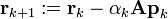
一般地，若已知点x(k)和搜索方向d(k)，则从x(k)出发，沿d(k)进行搜索，得到

x(k+1) = x(k) + λkd(k) ,

其中步长λk满足

f(x(k) + λkd(k)) = min f(x(k)+λd(k))。

此时可求出λk的显示表达

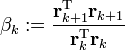
计算f(x)在x(k+1)处的梯度。若||gk+1|| = 0，则停止计算；否则，用-gk+1和d(k)构造下一个搜索方向d(k+1)，并使d(k+1)和d(k)关于A共轭。按此设想，令

d(k+1) = -gk+1 + βkd(k)，

上式两端左乘d(k)TA，并令

d(k)TAd(k+1) = -d(k)TAgk+1 + βkd(k)TAd(k) = 0，

由此得到

βk = d(k)TAgk+1 / d(k)TAd(k)。

再从x(k+1)出发，沿方向d(k+1)搜索。

在FR法中，初始搜索方向必须取最速下降方向，这一点决不可忽视。因子βk可以简化为：βk = ||gk+1||2 / ||gk||2。

实现算法如下：

The algorithm is detailed below for solving Ax = b where A is a real, symmetric, positive-definite matrix. The input vector x₀ can be an approximate initial solution or 0.

$.mathbf{r}_0 := .mathbf{b} - .mathbf{A x}_0 .,$ #x0为初始值向量

$.mathbf{p}_0 := .mathbf{r}_0 .,$

$k := 0 .,$

repeat

$.mathbf{x}_{k+1} := .mathbf{x}_k + .alpha_k .mathbf{p}_k .,$

$.mathbf{r}_{k+1} := .mathbf{r}_k - .alpha_k .mathbf{A p}_k .,$

if r_k+1 is sufficiently small then exit loop end

$.alpha_k := .frac{.mathbf{r}_k^.mathrm{T} .mathbf{r}_k}{.mathbf{p}_k^.mathrm{T} .mathbf{A p}_k} .,$

$.beta_k := .frac{.mathbf{r}_{k+1}^.mathrm{T} .mathbf{r}_{k+1}}{.mathbf{r}_k^.mathrm{T} .mathbf{r}_k} .,$

$.mathbf{p}_{k+1} := .mathbf{r}_{k+1} + .beta_k .mathbf{p}_k .,$

$k := k + 1 .,$

end repeat

The result is x_k+1

一个很容易理解的例子：

To illustrate the conjugate gradient method, we will complete a simple example.

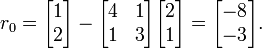
Considering the linear system Ax = b given by

$.mathbf{A} .mathbf{x}= .begin{bmatrix} 4 & 1 .. 1 & 3 .end{bmatrix}.begin{bmatrix} x_1 .. x_2 .end{bmatrix} = .begin{bmatrix} 1 .. 2 .end{bmatrix} ,$

we will perform two steps of the conjugate gradient method beginning with the initial guess

$.mathbf{x}_0 = .begin{bmatrix} 2 .. 1 .end{bmatrix}$

in order to find an approximate solution to the system.

[edit]Solution

Our first step is to calculate the residual vector r₀ associated with x₀. This residual is computed from the formula r₀ =b - Ax₀, and in our case is equal to

$r_0 = .begin{bmatrix} 1 .. 2 .end{bmatrix} - .begin{bmatrix} 4 & 1 .. 1 & 3 .end{bmatrix} .begin{bmatrix} 2 .. 1 .end{bmatrix} = .begin{bmatrix}-8 .. -3 .end{bmatrix}.$

Since this is the first iteration, we will use the residual vector r₀ as our initial search direction p₀; the method of selecting p_k will change in further iterations.

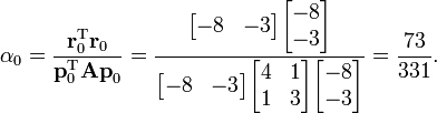
We now compute the scalar α₀ using the relationship

$.alpha_0 = .frac{.mathbf{r}_0^.mathrm{T} .mathbf{r}_0}{.mathbf{p}_0^.mathrm{T} .mathbf{A p}_0} = .frac{.begin{bmatrix} -8 & -3 .end{bmatrix} .begin{bmatrix} -8 .. -3 .end{bmatrix}}{ .begin{bmatrix} -8 & -3 .end{bmatrix} .begin{bmatrix} 4 & 1 .. 1 & 3 .end{bmatrix} .begin{bmatrix} -8 .. -3 .end{bmatrix} } = .frac{73}{331}.$

We can now compute x₁ using the formula

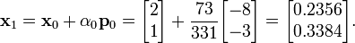
$.mathbf{x}_1 = .mathbf{x}_0 + .alpha_0.mathbf{p}_0 = .begin{bmatrix} 2 .. 1 .end{bmatrix} + .frac{73}{331} .begin{bmatrix} -8 .. -3 .end{bmatrix} = .begin{bmatrix} 0.2356 .. 0.3384 .end{bmatrix}.$

This result completes the first iteration, the result being an "improved" approximate solution to the system, x₁. We may now move on and compute the next residual vector r₁ using the formula

$.mathbf{r}_1 = .mathbf{r}_0 - .alpha_0 .mathbf{A} .mathbf{p}_0 = .begin{bmatrix} -8 .. -3 .end{bmatrix} - .frac{73}{331} .begin{bmatrix} 4 & 1 .. 1 & 3 .end{bmatrix} .begin{bmatrix} -8 .. -3 .end{bmatrix} = .begin{bmatrix} -0.2810 .. 0.7492 .end{bmatrix}.$

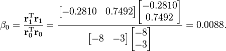
Our next step in the process is to compute the scalar β₀ that will eventually be used to determine the next search direction p₁.

$.beta_0 = .frac{.mathbf{r}_1^.mathrm{T} .mathbf{r}_1}{.mathbf{r}_0^.mathrm{T} .mathbf{r}_0} = .frac{.begin{bmatrix} -0.2810 & 0.7492 .end{bmatrix} .begin{bmatrix} -0.2810 .. 0.7492 .end{bmatrix}}{.begin{bmatrix} -8 & -3 .end{bmatrix} .begin{bmatrix} -8 .. -3 .end{bmatrix}} = 0.0088.$

Now, using this scalar β₀, we can compute the next search direction p₁ using the relationship

$.mathbf{p}_1 = .mathbf{r}_1 + .beta_0 .mathbf{p}_0 = .begin{bmatrix} -0.2810 .. 0.7492 .end{bmatrix} + 0.0088 .begin{bmatrix} -8 .. -3 .end{bmatrix} = .begin{bmatrix} -0.3511 .. 0.7229 .end{bmatrix}.$

We now compute the scalar α₁ using our newly-acquired p₁ using the same method as that used for α₀.

$.alpha_1 = .frac{.mathbf{r}_1^.mathrm{T} .mathbf{r}_1}{.mathbf{p}_1^.mathrm{T} .mathbf{A p}_1} = .frac{.begin{bmatrix} -0.2810 & 0.7492 .end{bmatrix} .begin{bmatrix} -0.2810 .. 0.7492 .end{bmatrix}}{ .begin{bmatrix} -0.3511 & 0.7229 .end{bmatrix} .begin{bmatrix} 4 & 1 .. 1 & 3 .end{bmatrix} .begin{bmatrix} -0.3511 .. 0.7229 .end{bmatrix} } = 0.4122.$

Finally, we find x₂ using the same method as that used to find x₁.

$.mathbf{x}_2 = .mathbf{x}_1 + .alpha_1 .mathbf{p}_1 = .begin{bmatrix} 0.2356 .. 0.3384 .end{bmatrix} + 0.4122 .begin{bmatrix} -0.3511 .. 0.7229 .end{bmatrix} = .begin{bmatrix} 0.0909 .. 0.6364 .end{bmatrix}.$

The result, x₂, is a "better" approximation to the system's solution than x₁ and x₀. If exact arithmetic were to be used in this example instead of limited-precision, then the exact solution would theoretically have been reached after n = 2 iterations (n being the order of the system).

共轭梯度法在R中的实现

在R的stats包中有个函数optim()可以实现该算法。该函数的使用如下：

optim(par, fn, gr = NULL, ...,

method = c("Nelder-Mead", "BFGS", "CG", "L-BFGS-B", "SANN"),

lower = -Inf, upper = Inf,

control = list(), hessian = FALSE)

该函数的默认方法是"Nelder-Mead"，可以通过指定"method"为"CG"来使用共轭梯度方法。该函数的参数"par"为初始值向量，参数"fn"为需要最小化的目标函数，它需要自己写。其他的参数可以见该函数的帮助文件。

参考自：

1 Wiki http://en.wikipedia.org/wiki/Conjugate_gradient_method

2 http://www.cnblogs.com/yangxi/archive/2011/10/20/2219408.html

3 CRAN

转载本文请联系原作者获取授权，同时请注明本文来自彭友松科学网博客。
链接地址：https://blog.sciencenet.cn/blog-54276-569356.html

上一篇：perl中十进制和16进制的转换
下一篇：R中用于排序的几个函数

收藏 IP: 159.226.118.*| 热度|

当前推荐数：1 推荐人：曾新林

该博文允许注册用户评论请点击登录评论 (2 个评论)

数据加载中...

返回顶部

博文发布时间已经超过87600小时，评论已关闭。

彭友松

扫一扫，分享此博文

高山流水分享 http://blog.sciencenet.cn/u/friendpine 走在科学路上的一位无名侠客，只是静静的走着.........

博文

对于共轭梯度最优化方法的一些认识

当前推荐数：1 推荐人：曾新林

该博文允许注册用户评论请点击登录评论 (2 个评论)

彭友松

全部作者的其他最新博文

全部精选博文导读

相关博文

高山流水分享 http://blog.sciencenet.cn/u/friendpine 走在科学路上的一位无名侠客，只是静静的走着.........

博文

对于共轭梯度最优化方法的一些认识

当前推荐数：1 推荐人： 曾新林

该博文允许注册用户评论 请点击登录 评论 (2 个评论)

彭友松

全部作者的其他最新博文

全部精选博文导读

相关博文

当前推荐数：1 推荐人：曾新林

该博文允许注册用户评论请点击登录评论 (2 个评论)