博文
翻车实录之Nature Medicine新冠单细胞文献|附全代码
||
大家好!我们又见面了,嘻嘻,今天我们来复现一篇于2020年5月12日深圳第三人民医院发表于nature medicine的新冠单细胞文献,这篇文章不久前我其实解读过,那时还在预印本medrxiv上,题为The landscape of lung bronchoalveolar immune cells in COVID-19 revealed by single-cell RNA sequencing,而发表在NM上的题目略有区别,Single-cell landscape of bronchoalveolar immune cells in patients with COVID-19。详细的解读分析请看第一篇新冠单细胞文献!|解读 ,废话不多说,开始吧!
下载数据
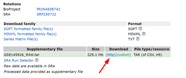
GEO datasets:GSE145926(http://www.ncbi.nlm.nih.gov/geo/query/acc.cgi?acc=GSE145926),点击下图标红处进行下载:
此时我们在作者原文中惊鸿一瞥,发现作者使用了13个sample,而在下载数据中只有12个,于是我们在metadata中发现作者使用了一个公共数据集:GSM3660650(https://www.ncbi.nlm.nih.gov/geo/query/acc.cgi?acc=GSM3660650),同样对下面3个文件进行下载:

加载R包
library(Seurat)
library(cowplot)
library(Matrix)
library(dplyr)
library(ggplot2)
library(reshape2)
加载数据
setwd("/DATA01/home/zhanghu/20200513covNATURE MEDICINE/GSE145926_RAW")
library(Seurat)#在下载文件中作者提供的均为.h5文件
C141<-Read10X_h5("GSM4339769_C141_filtered_feature_bc_matrix.h5")
C142<-Read10X_h5("GSM4339770_C142_filtered_feature_bc_matrix.h5")
C143<-Read10X_h5("GSM4339771_C143_filtered_feature_bc_matrix.h5")
C144<-Read10X_h5("GSM4339772_C144_filtered_feature_bc_matrix.h5")
C145<-Read10X_h5("GSM4339773_C145_filtered_feature_bc_matrix.h5")
C146<-Read10X_h5("GSM4339774_C146_filtered_feature_bc_matrix.h5")
C148<-Read10X_h5("GSM4475051_C148_filtered_feature_bc_matrix.h5")
C149<-Read10X_h5("GSM4475052_C149_filtered_feature_bc_matrix.h5")
C152<-Read10X_h5("GSM4475053_C152_filtered_feature_bc_matrix.h5")
C51<- Read10X_h5("GSM4475048_C51_filtered_feature_bc_matrix.h5")
C52<- Read10X_h5("GSM4475049_C52_filtered_feature_bc_matrix.h5")
C100<- Read10X_h5("GSM4475050_C100_filtered_feature_bc_matrix.h5")
GSM3660650<- Read10X(data.dir = '/DATA01/home/zhanghu/20200513covNATURE MEDICINE/GSE145926_RAW/GSM3660650')
构建seurat对象
C141<-CreateSeuratObject(counts = C141, project = "C141",min.cells = 3, min.features = 200)
C142<-CreateSeuratObject(counts = C142, project = "C142",min.cells = 3, min.features = 200)
C143<-CreateSeuratObject(counts = C143, project = "C143",min.cells = 3, min.features = 200)
C144<-CreateSeuratObject(counts = C144, project = "C144",min.cells = 3, min.features = 200)
C145<-CreateSeuratObject(counts = C145, project = "C145",min.cells = 3, min.features = 200)
C146<-CreateSeuratObject(counts = C146, project = "C146",min.cells = 3, min.features = 200)
C148<-CreateSeuratObject(counts = C148, project = "C148",min.cells = 3, min.features = 200)
C149<-CreateSeuratObject(counts = C149, project = "C149",min.cells = 3, min.features = 200)
C152<-CreateSeuratObject(counts = C152, project = "C152",min.cells = 3, min.features = 200)
C51<-CreateSeuratObject(counts = C51, project = "C51",min.cells = 3, min.features = 200)
C52<-CreateSeuratObject(counts = C52, project = "C52",min.cells = 3, min.features = 200)
C100<-CreateSeuratObject(counts = C100, project = "C100",min.cells = 3, min.features = 200)
GSM3660650<-CreateSeuratObject(counts = GSM3660650, project = "GSM3660650",min.cells = 3, min.features = 200)
分组
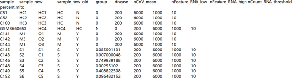
根据作者提供的meta.txt(https://github.com/zhangzlab/covid_balf/blob/master/meta.txt)对数据进行分组,一共4个健康(HC),3个轻症(M),6个重症(S)样本。
C141$group<-"mild"
C142$group<-"mild"
C143$group<-"severe"
C144$group<-"mild"
C145$group<-"severe"
C146$group<-"severe"
C148$group<-"severe"
C149$group<-"severe"
C152$group<-"severe"
C51$group <- "healthy"
C52$group <- "healthy"
C100$group <- "healthy"
GSM3660650$group <- "healthy"
查看细胞分布
#我们首先进行线粒体基因比例的提取,然后使用小提琴图对基因,转录本及线粒体比例进行展示
C141[["percent.mt"]]<-PercentageFeatureSet(C141,pattern = "^MT")
p141<-VlnPlot(C141, features = c("nFeature_RNA", "nCount_RNA", "percent.mt"), ncol = 3)
C142[["percent.mt"]]<-PercentageFeatureSet(C142,pattern = "^MT")
p142<-VlnPlot(C142, features = c("nFeature_RNA", "nCount_RNA", "percent.mt"), ncol = 3)
C143[["percent.mt"]]<-PercentageFeatureSet(C143,pattern = "^MT")
p143<-VlnPlot(C143, features = c("nFeature_RNA", "nCount_RNA", "percent.mt"), ncol = 3)
C144[["percent.mt"]]<-PercentageFeatureSet(C144,pattern = "^MT")
p144<-VlnPlot(C144, features = c("nFeature_RNA", "nCount_RNA", "percent.mt"), ncol = 3)
C145[["percent.mt"]]<-PercentageFeatureSet(C145,pattern = "^MT")
p145<-VlnPlot(C145, features = c("nFeature_RNA", "nCount_RNA", "percent.mt"), ncol = 3)
C146[["percent.mt"]]<-PercentageFeatureSet(C146,pattern = "^MT")
p146<-VlnPlot(C146, features = c("nFeature_RNA", "nCount_RNA", "percent.mt"), ncol = 3)
C148[["percent.mt"]]<-PercentageFeatureSet(C148,pattern = "^MT")
p148<-VlnPlot(C148, features = c("nFeature_RNA", "nCount_RNA", "percent.mt"), ncol = 3)
C149[["percent.mt"]]<-PercentageFeatureSet(C149,pattern = "^MT")
p149<-VlnPlot(C149, features = c("nFeature_RNA", "nCount_RNA", "percent.mt"), ncol = 3)
C152[["percent.mt"]]<-PercentageFeatureSet(C152,pattern = "^MT")
p152<-VlnPlot(C152, features = c("nFeature_RNA", "nCount_RNA", "percent.mt"), ncol = 3)
C51[["percent.mt"]]<-PercentageFeatureSet(C51,pattern = "^MT")
p51<-VlnPlot(C51, features = c("nFeature_RNA", "nCount_RNA", "percent.mt"), ncol = 3)
C52[["percent.mt"]]<-PercentageFeatureSet(C52,pattern = "^MT")
p52<-VlnPlot(C52, features = c("nFeature_RNA", "nCount_RNA", "percent.mt"), ncol = 3)
C100[["percent.mt"]]<-PercentageFeatureSet(C100,pattern = "^MT")
p100<-VlnPlot(C100, features = c("nFeature_RNA", "nCount_RNA", "percent.mt"), ncol = 3)
GSM3660650[["percent.mt"]]<-PercentageFeatureSet(GSM3660650,pattern = "^MT")
pGSM3660650<-VlnPlot(GSM3660650, features = c("nFeature_RNA", "nCount_RNA", "percent.mt"), ncol = 3)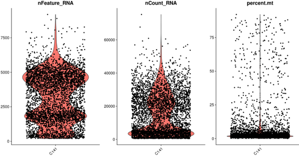
此时我们会出现无数张这样的图(可视化之为什么要使用箱线图?),我不去解释里面的意义了,我只谈一下第一张图中发现有两个细胞聚集“肚子”,我也其实出现过这样的分布图,于是有人说这可能是污染,上面细胞是下面细胞基因数的两倍,我其实大概率认为不太会出现这样的情况,原因(1)细胞数太多了,这建库质量得差到一定程度呢;(2)转录本并没有像基因数那样呈现双峰;(3)可以试一试去除doublet的工具(单细胞预测Doublets软件包汇总-过渡态细胞是真的吗?)啊,仅仅通过这个图下结论不太合适;(4)该样本可能是刺激样本,部分细胞受到刺激后的反应。
QC
我们按照文章中所给出的条件对细胞和基因进行筛选,原文:The following criteria were then applied to each cell of all nine patients and four healthy controls: gene number between 200 and 6,000, UMI count > 1,000 and mitochondrial gene percentage < 0.1.
C141 <- subset(C141, subset = nFeature_RNA > 200 & nFeature_RNA < 6000 & percent.mt < 10 & nCount_RNA >1000)
C142 <- subset(C142, subset = nFeature_RNA > 200 & nFeature_RNA < 6000 & percent.mt < 10 & nCount_RNA >1000)
C143 <- subset(C143, subset = nFeature_RNA > 200 & nFeature_RNA < 6000 & percent.mt < 10 & nCount_RNA >1000)
C144 <- subset(C144, subset = nFeature_RNA > 200 & nFeature_RNA < 6000 & percent.mt < 10 & nCount_RNA >1000)
C145 <- subset(C145, subset = nFeature_RNA > 200 & nFeature_RNA < 6000 & percent.mt < 10 & nCount_RNA >1000)
C146 <- subset(C146, subset = nFeature_RNA > 200 & nFeature_RNA < 6000 & percent.mt < 10 & nCount_RNA >1000)
C148 <- subset(C148, subset = nFeature_RNA > 200 & nFeature_RNA < 6000 & percent.mt < 10 & nCount_RNA >1000)
C149 <- subset(C149, subset = nFeature_RNA > 200 & nFeature_RNA < 6000 & percent.mt < 10 & nCount_RNA >1000)
C152 <- subset(C152, subset = nFeature_RNA > 200 & nFeature_RNA < 6000 & percent.mt < 10 & nCount_RNA >1000)
C51 <- subset(C51, subset = nFeature_RNA > 200 & nFeature_RNA < 6000 & percent.mt < 10 & nCount_RNA >1000)
C52 <- subset(C52, subset = nFeature_RNA > 200 & nFeature_RNA < 6000 & percent.mt < 10 & nCount_RNA >1000)
C100 <- subset(C100, subset = nFeature_RNA > 200 & nFeature_RNA < 6000 & percent.mt < 10 & nCount_RNA >1000)
GSM3660650 <- subset(GSM3660650, subset = nFeature_RNA > 200 & nFeature_RNA < 6000 & percent.mt < 10 & nCount_RNA >1000)
归一化
C141 <- NormalizeData(C141)
C142 <- NormalizeData(C142)
C143 <- NormalizeData(C143)
C144 <- NormalizeData(C144)
C145 <- NormalizeData(C145)
C146 <- NormalizeData(C146)
C148 <- NormalizeData(C148)
C149 <- NormalizeData(C149)
C152 <- NormalizeData(C152)
C51 <- NormalizeData(C51)
C52 <- NormalizeData(C52)
C100 <- NormalizeData(C100)
GSM3660650<- NormalizeData(GSM3660650)
计算高变基因
C141 <- FindVariableFeatures(C141, selection.method = "vst", nfeatures = 2000)
C142 <- FindVariableFeatures(C142, selection.method = "vst", nfeatures = 2000)
C143 <- FindVariableFeatures(C143, selection.method = "vst", nfeatures = 2000)
C144 <- FindVariableFeatures(C144, selection.method = "vst", nfeatures = 2000)
C145 <- FindVariableFeatures(C145, selection.method = "vst", nfeatures = 2000)
C146 <- FindVariableFeatures(C146, selection.method = "vst", nfeatures = 2000)
C148 <- FindVariableFeatures(C148, selection.method = "vst", nfeatures = 2000)
C149 <- FindVariableFeatures(C149, selection.method = "vst", nfeatures = 2000)
C152 <- FindVariableFeatures(C152, selection.method = "vst", nfeatures = 2000)
C51 <- FindVariableFeatures(C51, selection.method = "vst", nfeatures = 2000)
C52 <- FindVariableFeatures(C52, selection.method = "vst", nfeatures = 2000)
C100 <- FindVariableFeatures(C100, selection.method = "vst", nfeatures = 2000)
GSM3660650 <- FindVariableFeatures(GSM3660650, selection.method = "vst", nfeatures = 2000)
数据整合
sample.anchors <- FindIntegrationAnchors(object.list = list(C141,C142,C143,C144,C145,C146,C148,C149,C152,C51,C52,C100,GSM3660650 ), dims = 1:50)
sample.combined <- IntegrateData(anchorset = sample.anchors, dims = 1:50)
由于数据量较大,该步骤会需要大量时间,建议去买根冰棍,溜达一圈或者打局王者荣耀。。。我的安琪拉!

大约2个小时后。。。。。。
加载样本信息
其中作者将样本信息记录在https://github.com/zhangzlab/covid_balf/blob/master/meta.txt上:
samples = read.delim2("meta.txt",header = TRUE, stringsAsFactors = FALSE,check.names = FALSE, sep = "\t")
sample_info = as.data.frame(colnames(nCoV.integrated))
colnames(sample_info) = c('ID')
rownames(sample_info) = sample_info$ID
sample_info$sample = nCoV.integrated@meta.data$orig.ident
sample_info = dplyr::left_join(sample_info,samples)
rownames(sample_info) = sample_info$ID
nCoV.integrated = AddMetaData(object = nCoV.integrated, metadata = sample_info)
对整合数据进行归一化和标准化
原文中在数据整合后的处理:The filtered gene-barcode matrix was first normalized using ‘LogNormalize’ methods in Seurat v.3 with default parameters. The top 2,000 variable genes were then identified using the ‘vst’ method in Seurat FindVariableFeatures function. Variables ‘nCount_RNA’ and ‘percent.mito’ were regressed out in the scaling step and PCA was performed using the top 2,000 variable genes. 按照以上说明进行操作。
DefaultAssay(nCoV.integrated) <- "RNA"
nCoV.integrated[['percent.mito']] <- PercentageFeatureSet(nCoV.integrated, pattern = "^MT-")
nCoV.integrated <- NormalizeData(object = nCoV.integrated, normalization.method = "LogNormalize", scale.factor = 1e4)
nCoV.integrated <- FindVariableFeatures(object = nCoV.integrated, selection.method = "vst", nfeatures = 2000,verbose = FALSE)
nCoV.integrated <- ScaleData(nCoV.integrated, verbose = FALSE, vars.to.regress = c("nCount_RNA", "percent.mito"))
VlnPlot(object = nCoV.integrated, features = c("nFeature_RNA", "nCount_RNA"), ncol = 2)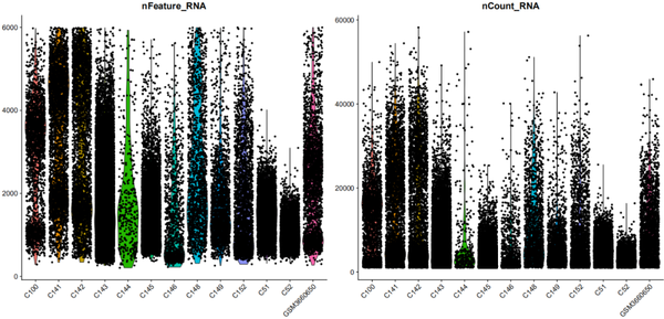
我们其实也可以看出不同样本之间的差异性还是挺大的,比如C100,C51,C52以及GSMXXX都是正常人,但我们也同时发现他们的基因和转录本表达的集中程度也是不相同的。当然C144细胞数较少显而易见。
FeatureScatter(object = nCoV.integrated, feature1 = "nCount_RNA", feature2 = "nFeature_RNA")
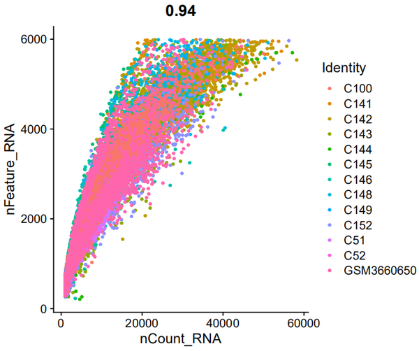
相关性很好哦。。。。
PCA
nCoV.integrated <- ScaleData(nCoV.integrated, verbose = FALSE, vars.to.regress = c("nCount_RNA", "percent.mito"))
nCoV.integrated <- RunPCA(nCoV.integrated, verbose = FALSE,npcs = 100)
nCoV.integrated <- ProjectDim(object = nCoV.integrated)
ElbowPlot(object = nCoV.integrated,ndims = 100)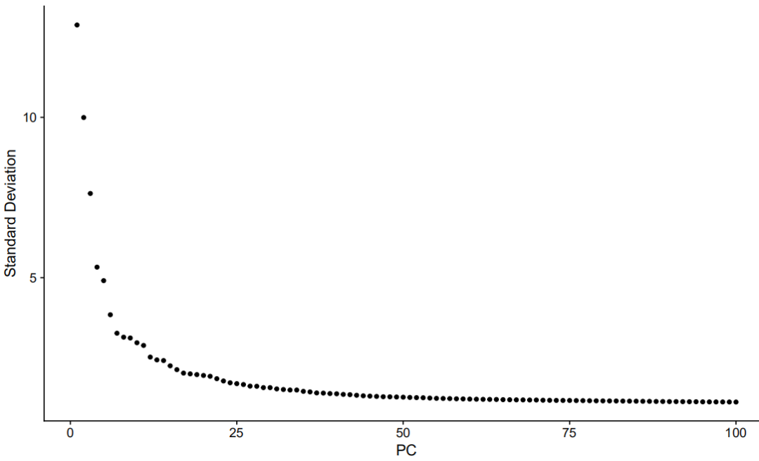
聚类
###cluster
nCoV.integrated <- FindNeighbors(object = nCoV.integrated, dims = 1:50)
nCoV.integrated <- FindClusters(object = nCoV.integrated, resolution = 1.2)
可视化
nCoV.integrated <- RunTSNE(object = nCoV.integrated, dims = 1:50)
DimPlot(object = nCoV.integrated, reduction = 'tsne',label = TRUE)
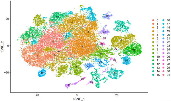
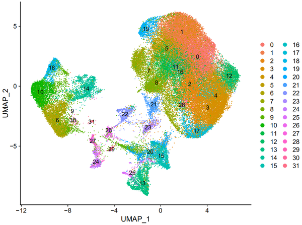
我们可以看到一共分为了32个cluster,命名为cluster0-31。使用umap进行展示:
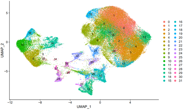
All seems like rather fine , but,此时我们来看原图:
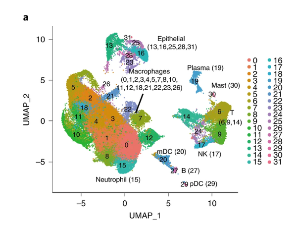
原图fig1
还是有一点点区别的,可能是随机种子什么的问题,anyway,分群确实也是蛮像的。
查找高变标记基因
DefaultAssay(nCoV.integrated) <- "RNA"
# find markers for every cluster compared to all remaining cells, report only the positive ones
nCoV.integrated@misc$markers <- FindAllMarkers(object = nCoV.integrated, assay = 'RNA',only.pos = TRUE, test.use = 'MAST')
write.table(nCoV.integrated@misc$markers,file='marker_MAST.txt',row.names = FALSE,quote = FALSE,sep = '\t')
VlnPlot(object = nCoV.integrated, features = c("nFeature_RNA", "nCount_RNA"))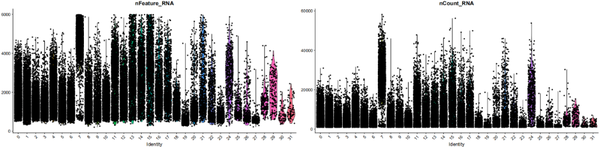
我们使用小提琴图看每个cluster中基因和转录本的分布,一般情况我们其实啥也看不出来的,但上图我们可以明显看出cluster 7在基因水平和转录本水平均较高,他是什么,他为什么这样呢,他是doublet吗?
不同组之间的对比
由于作者先期已经使用每个cluster中的高变基因鉴定出了每种细胞类型,我们这里直接使用marker进行分析。
markers = c('AGER','SFTPC','SCGB3A2','TPPP3','KRT5',
            'CD68','FCN1','CD1C','TPSB2','CD14','MARCO','CXCR2',
            'CLEC9A','IL3RA',
            'CD3D','CD8A','KLRF1',
            'CD79A','IGHG4','MS4A1',
            'VWF','DCN',
            'FCGR3A','TREM2','KRT18')
hc.markers=nCoV.integrated@misc$markers
hc.markers %>% group_by(cluster) %>% top_n(n = 30, wt = avg_logFC) -> top30
var.genes = c(nCoV.integrated@assays$RNA@var.features,top30$gene,markers)
nCoV.integrated <- ScaleData(nCoV.integrated, verbose = FALSE, vars.to.regress = c("nCount_RNA", "percent.mito"),features = var.genes)其实作者使用的以上操作也是我第一次见,我们看作者干了什么?首先作者通过高变基因把cluster中的marker挑了出来,然后top30高变基因,然后把var.features和他们结合在一起作为var.genes,共同进行标准化,我们来使用?ScaleData查看一下features的涵义:
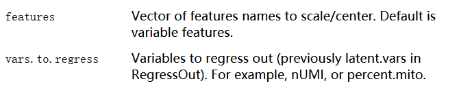
也就是说对features进行标准化呗。
DimPlot(object = nCoV.integrated, reduction = 'umap',label = TRUE)
DimPlot(object = nCoV.integrated, reduction = 'umap',label = FALSE, group.by = 'sample_new')
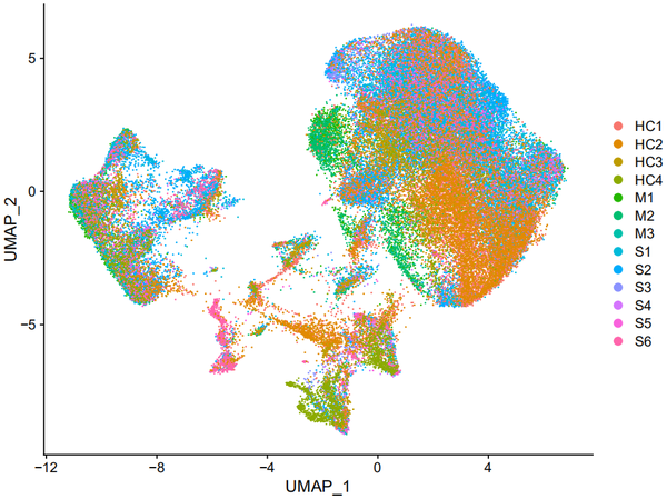
从上图我们其实可以看出,各个样本之间的重合度还是蛮高的,也可以看出某些cluster在某些样本中的比例较高。
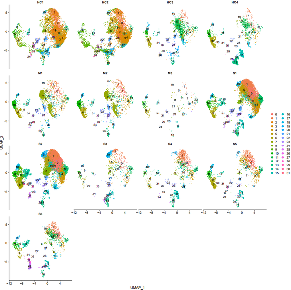
DimPlot(object = nCoV.integrated, reduction = 'umap',label = TRUE, split.by = 'sample_new', ncol = 4)
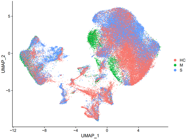
DimPlot(object = nCoV.integrated, reduction = 'umap',label = FALSE, group.by = 'group')
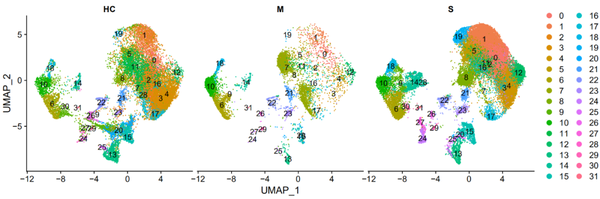
DimPlot(object = nCoV.integrated, reduction = 'umap',label = TRUE, split.by = 'group', ncol = 3)
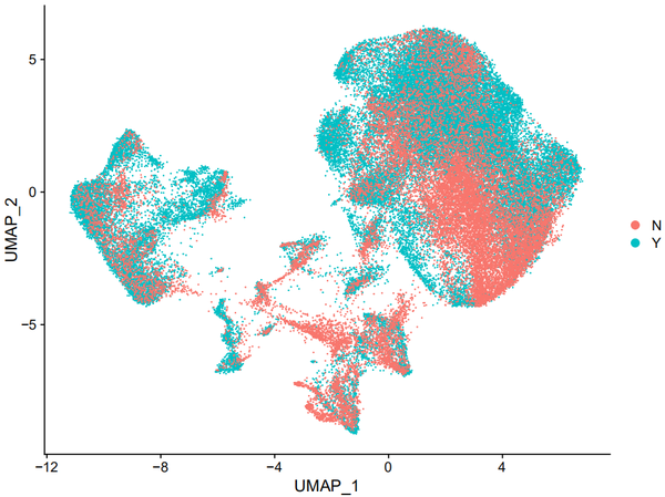
DimPlot(object = nCoV.integrated, reduction = 'umap',label = FALSE, group.by = 'disease')
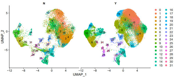
DimPlot(object = nCoV.integrated, reduction = 'umap',label = TRUE, split.by = 'disease', ncol = 2)
细胞分型
markers = c('TPPP3','KRT18','CD68','FCGR3B','CD1C','CLEC9A','LILRA4','TPSB2','CD3D','KLRD1','MS4A1','IGHG4')很熟悉吧!我们首先来看一下这些marker所对应的细胞类型,根据作者在Extended Data Fig.1中的描述,发现TPP3是Ciliated,KRT18是Secretory,CD68是Macrophages,FCGR3B是Neutrophil,CD1C是mDC,LILRA4是pDC,TPSB2是Mast cell,CD3D是T cell,KLRD1是NK cell,MS4A1是B cell,IGHG4是Plasma cell,在doublets中表达CD68和CD3D。
pp_temp = FeaturePlot(object = nCoV.integrated, features = markers,cols = c("lightgrey","#ff0000"),combine = FALSE)
 plots <- lapply(X = pp_temp, FUN = function(p) p + theme(axis.title = element_text(size = 18),axis.text = element_text(size = 18),plot.title = element_text(family = 'sans',face='italic',size=20),legend.text = element_text(size = 20),legend.key.height = unit(1.8,"line"),legend.key.width = unit(1.2,"line") ))
  pp = CombinePlots(plots = plots,ncol = 4,legend = 'right')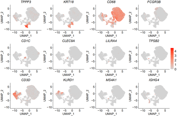
哈哈哈哈,以上可以看出这些marker的特异性还是蛮好的。
我们来看一下原图吧:
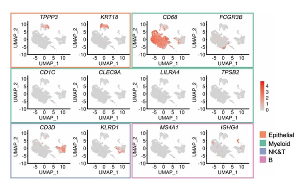
Extended Data Fig.1
绘制点图:
  pp = DotPlot(nCoV.integrated, features = rev(markers),cols = c('white','#F8766D'),dot.scale =5) + RotatedAxis()
  pp = pp + theme(axis.text.x = element_text(size = 12),axis.text.y = element_text(size = 12)) + labs(x='',y='') + guides(color = guide_colorbar(title = 'Scale expression'),size = guide_legend(title = 'Percent expressed')) + theme(axis.line = element_line(size = 0.6))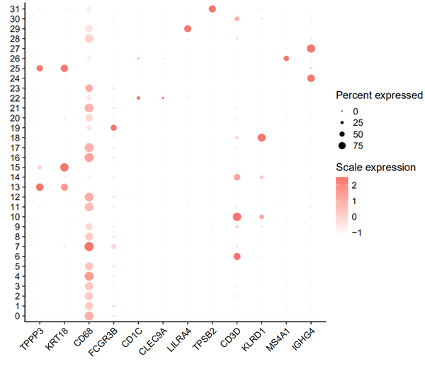
其实我复现的和作者的分群是略有区别的,但也不影响分析,anyway,我们仿照作者进行分群,在Epithelial中TPPP3-Ciliated(13,25),KRT18(15),Myeloid中CD68-Macrophages(0、1、2、3、4、5、7、8、9、11、12、16、17、20、21、23、28),FCGR3B-Neutrophil(19),CD1C-mDC(22),LILRA4-pDC(29),TPSB2-Mast cell(31),NK&T中CD3D-T cell(6、10、30),KLRD1-NK cell(18),B中MS4A1-B cell(26),IGHG4-Plasma cell(24,27),others中CD68&CD3D-Doublets(14)。OK,我们来看一下原图吧:
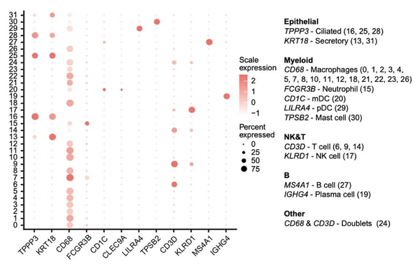
Extended Data Fig.1
绘制比例图
library(ggplot2)
nCoV.integrated[["cluster"]] <- Idents(object = nCoV.integrated)
big.cluster = nCoV.integrated@meta.data
organ.summary = table(big.cluster$sample_new,big.cluster$cluster)
write.table(organ.summary,file = '1-nCoV-percentage-sample.txt',quote = FALSE,sep = '\t')
library(ggplot2)
library(dplyr)
library(reshape2)
organ.summary = read.delim2("1-nCoV-percentage-sample.txt",header = TRUE, stringsAsFactors = FALSE,check.names = FALSE, sep = "\t")
organ.summary$group = rownames(organ.summary)
organ.summary.dataframe = melt(organ.summary)
colnames(organ.summary.dataframe) = c('group','cluster','cell')
samples_name_new = c('HC1','HC2','HC3','HC4','M1','M2','M3','S1','S2','S3','S4','S5','S6')
organ.summary.dataframe$group = factor(organ.summary.dataframe$group,labels = samples_name_new,levels = samples_name_new)
organ.summary.dataframe$cell = as.numeric(organ.summary.dataframe$cell)
作者上面的这顿操作真是猛如虎。。。
准备完数据后,准备画图:
new_order = c('0','1','2','3','4','5','7','8','9','11','12','16','17','20','21','23','28','19','24','27','13','25','15','6','10','30','18','22','26','29','31','14')
  organ.summary.dataframe$cluster = factor(organ.summary.dataframe$cluster,levels = new_order,labels = new_order)
  cols = c('#32b8ec','#60c3f0','#8ccdf1','#cae5f7','#92519c','#b878b0','#d7b1d2','#e7262a','#e94746','#eb666d','#ee838f','#f4abac','#fad9d9')
  pp = ggplot(data=organ.summary.dataframe, aes(x=cluster, y=cell, fill=group)) + geom_bar(stat="identity",width = 0.6,position=position_fill(reverse = TRUE),size = 0.3,colour = '#222222') + labs(x='',y='Fraction of sample per cluster (%)') +
    theme(axis.title.x = element_blank(),axis.text = element_text(size = 16),axis.title.y =element_text(size = 16), legend.text = element_text(size = 15),legend.key.height = unit(5,'mm'),
          legend.title = element_blank(),panel.grid.minor = element_blank()) + cowplot::theme_cowplot() + theme(axis.text.x = element_text(size = 10)) +
    scale_fill_manual(values = cols)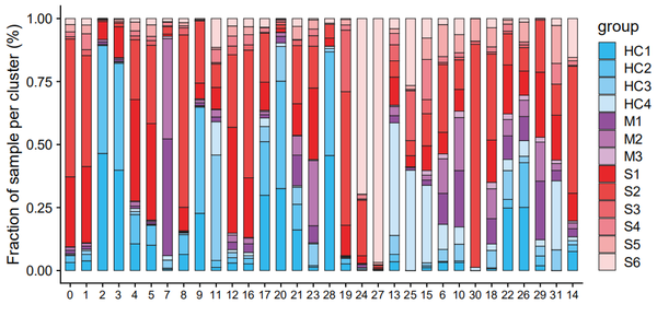
细胞命名
 nCoV.integrated1 <- RenameIdents(object = nCoV.integrated,
                                   '13' = 'Epithelial','15' = 'Epithelial','25' = 'Epithelial',                                '0'='Macrophages','1'='Macrophages','2'='Macrophages','3'='Macrophages','4'='Macrophages','5'='Macrophages','7'='Macrophages','8'='Macrophages','9'='Macrophages','11'='Macrophages','12'='Macrophages','16'='Macrophages','17'='Macrophages','20'='Macrophages','21'='Macrophages','23'='Macrophages','28'='Macrophages',
                                   '31'='Mast',
                                   '6'='T','10'='T','30'='T',
                                   '18'='NK',
                                   '24'='Plasma','27'='Plasma',
                                   '26'='B',
                                   '19'='Neutrophil',
                                   '22'='mDC',
                                   '29'='pDC',
                                   '14'='Doublets')
#去除doublets
  nCoV.integrated1$celltype = Idents(nCoV.integrated1)
  nCoV.integrated1 = subset(nCoV.integrated1,subset = celltype != 'Doublets')
  nCoV_groups = c('Epithelial','Macrophages','Neutrophil','mDC','pDC','Mast','T','NK','B','Plasma')
  nCoV.integrated1$celltype = factor(nCoV.integrated1$celltype,levels = nCoV_groups,labels = nCoV_groups)
Idents(nCoV.integrated1) = nCoV.integrated1$celltype细胞命名后的dimplot:
pp_temp = DimPlot(object = nCoV.integrated1, reduction = 'umap',label = FALSE, label.size = 6,split.by = 'group', ncol = 3,repel = TRUE,combine = TRUE)
 pp_temp = pp_temp + theme(axis.title = element_text(size = 17),axis.text = element_text(size = 17),strip.text = element_text(family = 'arial',face='plain',size=17), legend.text = element_text(size = 17),axis.line = element_line(size = 1),axis.ticks = element_line(size = 0.8),legend.key.height = unit(1.4,"line"))
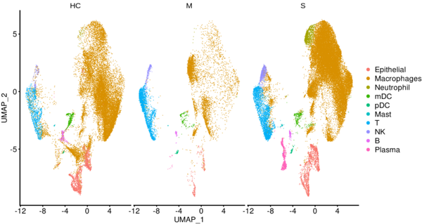
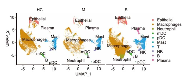
Extended Data Fig.1(原图)
按照sample进行分类:
 pp_temp = DimPlot(object = nCoV.integrated1, reduction = 'umap',label = FALSE, split.by = 'sample_new', label.size = 7,ncol = 5,repel = TRUE, combine = TRUE,pt.size = 1.5)
  pp_temp = pp_temp + theme(axis.title = element_text(size = 22),axis.text = element_text(size = 22),strip.text = element_text(family = 'sans',face='plain',size=22),legend.text = element_text(size = 22),legend.key.height = unit(1.8,"line"),legend.key.width = unit(1.2,"line"),axis.line = element_line(size = 1.2),axis.ticks = element_line(size = 1.2))
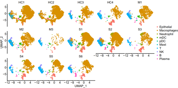
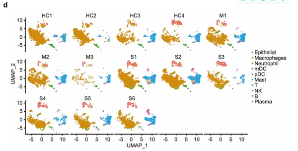
Extended Data Fig.1(原图)
等等!!!!!!
此时我发现了一个我的重大失误!就是我的细胞分群错了。。。。。。哭出声来!!! 通过featureplot并结合作者原文其实可以看出cluster9是doublets,cluster14是T细胞。。。。 于是应该是这个样子的:

剩下的我就不重来一遍的,我太难了。。。。 up to now,我基本已经把作者的细胞大群复现完了,你也可以使用作者的github上的上传代码进行复现,不过前期我确实没有看懂,所以就是按照自己结合原文的意思进行复现的。。。
不行了我要去玩耍了,这篇文献没有几页,但我估计已经看了N遍了。。。。
参考文献
Liao M, Liu Y, Yuan J, Wen Y, Xu G, Zhao J, Cheng L, Li J, Wang X, Wang F, Liu L, Amit I, Zhang S, Zhang Z. Single-cell landscape of bronchoalveolar immune cells in patients with COVID-19. Nat Med. 2020 May 12. doi:10.1038
Code
https://github.com/zhangzlab/covid_balf
你可能还想看


https://blog.sciencenet.cn/blog-118204-1234932.html
上一篇:整合基因组学和蛋白质结构的致病机制分析
下一篇:一个R包完成单细胞基因集富集分析 (全代码)